02b · One refractiveindex.info model, every engine

02_technology showed that the engines’ shipped material models agree with refractiveindex.info. This notebook takes a real measured model straight from refractiveindex.info — its full complex, wavelength-dependent n(λ) + i·k(λ) — and feeds that exact model into each FDTD engine.

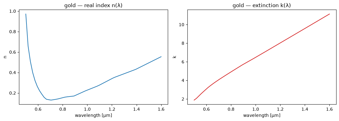
The material is gold (Johnson & Christy 1972) — a strongly dispersive, strongly lossy material where the imaginary part carries real weight (k runs from ~3 in the visible to ~11 in the near-IR). If a model is going to break on the trip into an engine, it breaks here.

from pathlib import Path

import matplotlib.pyplot as plt
import numpy as np

from gds_fdtd.materials.rii import load_rii_material


def _find(rel: str) -> Path:
    for base in (Path.cwd(), *Path.cwd().parents):
        if (base / rel).exists():
            return base / rel
    raise FileNotFoundError(rel)


RII_DB = _find("examples/02_technology/rii_db")
C = 299_792_458.0

au = load_rii_material("main", "Au", "Johnson", db_dir=str(RII_DB))
lo, hi = au.wavelength_range_um
WL = np.linspace(max(lo, 0.5), min(hi, 1.6), 60)
n_rii = np.asarray(au.n_at(WL))
k_rii = np.asarray(au.k_at(WL))
print(f"gold (Johnson): tabulated {lo:.3f}–{hi:.3f} µm; "
      f"@1.55 µm n+ik = {au.n_at(1.55):.3f} + {au.k_at(1.55):.3f}i")

gold (Johnson): tabulated 0.188–1.937 µm; @1.55 µm n+ik = 0.524 + 10.742i

The model

This is what we’re going to feed to the engines — the measured optical constants, dispersive in both the real and imaginary parts.

fig, (axn, axk) = plt.subplots(1, 2, figsize=(11, 4))
axn.plot(WL, n_rii, color="C0")
axn.set(xlabel="wavelength [µm]", ylabel="n", title="gold — real index n(λ)")
axk.plot(WL, k_rii, color="C3")
axk.set(xlabel="wavelength [µm]", ylabel="k", title="gold — extinction k(λ)")
fig.tight_layout()
plt.show()

tidy3d — fit to a dispersive medium

RiiMaterial.to_tidy3d_medium() fits the tabulated n, k to a pole-residue dispersive medium you drop straight into a td.Simulation. We evaluate the fitted medium back over the band and overlay it on the input.

import tidy3d as td  # noqa: E402

medium = au.to_tidy3d_medium(wavelength_um=WL, max_num_poles=6)
nk_td = np.array([[float(x) for x in medium.nk_model(C / (w * 1e-6))] for w in WL])
print(f"tidy3d dispersive medium: max |Δn|={np.max(np.abs(nk_td[:, 0] - n_rii)):.3f}, "
      f"max |Δk|={np.max(np.abs(nk_td[:, 1] - k_rii)):.3f}")

22:35:55 PDT WARNING: Using canonical configuration directory at                
             '/home/mustafa/.config/tidy3d'. Found legacy directory at          
             '~/.tidy3d', which will be ignored. Remove it manually or run      
             'tidy3d config migrate --delete-legacy' to clean up.               

22:36:03 PDT WARNING: Unable to fit with weighted RMS error under               
             'tolerance_rms' of 1e-05                                           

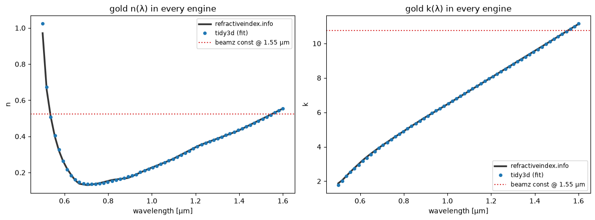
tidy3d dispersive medium: max |Δn|=0.052, max |Δk|=0.106

Lumerical — a sampled material

Lumerical takes the model as a sampled material: the (frequency, permittivity) table itself. It stores the data verbatim, so it reproduces the refractiveindex.info model almost exactly. (Needs a Lumerical license; skipped gracefully without one.)

nk_lum = None
try:
    import lumapi

    f_hz = C / (WL * 1e-6)
    eps = (n_rii + 1j * k_rii) ** 2
    fdtd = lumapi.FDTD(hide=True)
    name = fdtd.addmaterial("Sampled 3D data")
    fdtd.setmaterial(name, "sampled data", np.column_stack([f_hz, eps]))
    nk_lum = np.array([complex(np.asarray(fdtd.getindex(name, float(fi))).ravel()[0]) for fi in f_hz])
    nk_lum = np.column_stack([nk_lum.real, np.abs(nk_lum.imag)])
    fdtd.close()
    print(f"lumerical sampled material: max |Δn|={np.max(np.abs(nk_lum[:, 0] - n_rii)):.4f}, "
          f"max |Δk|={np.max(np.abs(nk_lum[:, 1] - k_rii)):.4f}")
except Exception as e:  # noqa: BLE001 - license optional
    print(f"(Lumerical not available — skipping: {e})")

(Lumerical not available — skipping: 'appOpen error: \n Failed to start messaging, check licenses...Error: Could not connect to Ansys license server specified at 27025@ansys-rlm.ece.ubc.ca<br>Would you like to reconfigure your license settings?, Response: Yes\n')

beamz — a single index (v1)

beamz v1 models each material as one constant n + ik, so a dispersive model collapses to its value at your design wavelength. Fine for a narrow band; just know it does not disperse.

DESIGN_WL = 1.55
nk_beamz = complex(au.nk_at(DESIGN_WL))
print(f"beamz constant @ {DESIGN_WL} µm: n + ik = {nk_beamz.real:.3f} + {nk_beamz.imag:.3f}i")

beamz constant @ 1.55 µm: n + ik = 0.524 + 10.742i

The whole model, in every engine

The refractiveindex.info model (solid), the tidy3d fit (dots), the Lumerical sampled material (dashes), and the beamz constant (flat). tidy3d and Lumerical carry the full complex dispersion; beamz pins a single point.

fig, (axn, axk) = plt.subplots(1, 2, figsize=(12, 4.5))
for ax, comp, rii, lab in ((axn, 0, n_rii, "n"), (axk, 1, k_rii, "k")):
    ax.plot(WL, rii, "-", lw=2.5, color="0.2", label="refractiveindex.info")
    ax.plot(WL, nk_td[:, comp], "o", ms=4, color="C0", label="tidy3d (fit)")
    if nk_lum is not None:
        ax.plot(WL, nk_lum[:, comp], "--", lw=1.5, color="C1", label="Lumerical (sampled)")
    ax.axhline((nk_beamz.real, nk_beamz.imag)[comp], ls=":", color="C3",
               label=f"beamz const @ {DESIGN_WL} µm")
    ax.set(xlabel="wavelength [µm]", ylabel=lab, title=f"gold {lab}(λ) in every engine")
    ax.legend(fontsize="small")
fig.tight_layout()
plt.show()

Using it in a simulation

to_tidy3d_medium() returns a real td.Medium you can assign to any structure, and the Lumerical sampled material is a named material like any other — so a device built with a refractiveindex.info model runs exactly like one built with a vendor model:

medium = load_rii_material("main", "Si", "Salzberg").to_tidy3d_medium()
structure = td.Structure(geometry=..., medium=medium)   # dispersive Si, from rii

Doing this from the technology file

You rarely call these by hand. In the tech file, give a material an rii: reference and (optionally) source: rii, and every engine builds its material from that model automatically — tidy3d a dispersive medium, Lumerical a sampled material, beamz a constant.

The shared examples/tech.yaml does this live: its substrate carries all three sources and pins source: rii, so the buried oxide comes from the Malitson (1965) Sellmeier page no matter which engine runs the job:

materials:
  SiO2_rii:
    nk: 1.444                          # neutral constant fallback
    tidy3d: 1.444                      # eda source, tidy3d flavor
    lumerical: SiO2 (Glass) - Palik    # eda source, Lumerical flavor
    rii: {shelf: main, book: SiO2, page: Malitson}
    source: rii        # <- overrides the eda→rii→nk precedence on EVERY engine

substrate: {z_base: 0.0, z_span: -2, material: SiO2_rii}

select_source is the function every engine calls to make this choice — ask it directly what each one would do:

from gds_fdtd.materials.select import select_source  # noqa: E402
from gds_fdtd.technology import Technology  # noqa: E402

tech = Technology.from_yaml(_find("examples/tech.yaml"))
d = tech.to_solver_dict()
substrate = d["substrate"][0]["material"]
superstrate = d["superstrate"][0]["material"]

print(f"{'material':12s}  {'tidy3d':10s}  {'lumerical':10s}  {'beamz':10s}")
for label, mat in [("substrate", substrate), ("superstrate", superstrate)]:
    picks = [select_source(mat, eng, name=label) for eng in ("tidy3d", "lumerical", "beamz")]
    print(f"{label:12s}  {picks[0]:10s}  {picks[1]:10s}  {picks[2]:10s}")

material      tidy3d      lumerical   beamz     
substrate     rii         rii         rii       
superstrate   eda         eda         nk

The superstrate (no source: pin) shows the default precedence: engines with a vendor database use it (eda), beamz falls through to nk. The pinned substrate answers rii everywhere. On tidy3d that buys real dispersion — the medium built from the tech file is a Sellmeier fit, not a constant:

import os  # noqa: E402

os.environ["GDS_FDTD_RII_DB"] = str(RII_DB)  # engines that build the substrate need the DB

sio2 = tech.substrate.material.rii.load()  # the named material, resolved onto the layer
medium = sio2.to_tidy3d_medium(wavelength_um=np.linspace(1.5, 1.6, 11))
wl = np.array([1.50, 1.55, 1.60])
n_fit = np.sqrt(medium.eps_model(td.C_0 / wl)).real
for w, n_r in zip(wl, n_fit, strict=True):
    print(f"λ={w:.2f} µm   rii n={sio2.n_at(w):.6f}   tidy3d medium n={n_r:.6f}")

λ=1.50 µm   rii n=1.444618   tidy3d medium n=1.444639
λ=1.55 µm   rii n=1.444024   tidy3d medium n=1.444010
λ=1.60 µm   rii n=1.443419   tidy3d medium n=1.443440

The selection rule (per material, per engine) is eda → rii → nk, with source: as an explicit override and a clear error if nothing applies — see docs/technology.rst → Material sources.

Recap

A refractiveindex.info page is a portable, engine-independent source of truth: its full n(λ) + i·k(λ) flows into tidy3d (a dispersion fit) and Lumerical (a sampled material) intact, and into beamz as a single-wavelength constant. Pin it with source: rii — as the shipped tech file does for its substrate — and every engine models that material from the same measured page.