04 · Reading results — everything an `SMatrix` tells you¶

Every engine returns the same object: a canonical SMatrix (complex, multi-port, multi-mode). This notebook is a tour of what you can read from it — magnitudes, loss, phase, the physical sanity checks, and file I/O — all offline and free (we load a recorded y-branch result, no engine needed).

from pathlib import Path

import matplotlib.pyplot as plt
import numpy as np

from gds_fdtd.plotting import plot_smatrix, smatrix_summary
from gds_fdtd.smatrix import SMatrix


def _find(rel: str) -> Path:
    for base in (Path.cwd(), *Path.cwd().parents):
        if (base / rel).exists():
            return base / rel
    raise FileNotFoundError(rel)


sm = SMatrix.from_npz(str(_find("examples/07_choosing_an_engine/recorded/ybranch_tidy3d.npz")))
print(f"{sm.name}: {sm.n_ports} ports {sm.port_names}, {sm.n_modes} mode(s), "
      f"{sm.wavelength_um.size} wavelengths {sm.wavelength_um.min():.3f}–{sm.wavelength_um.max():.3f} µm")

ebeam_y_1550: 3 ports ['opt1', 'opt2', 'opt3'], 1 mode(s), 5 wavelengths 1.500–1.600 µm

1 · The raw array¶

Under the hood sm.s is a complex array indexed [wavelength, out, in, mode_out, mode_in]. You rarely touch it directly — sm.sel(out, in_, ...) pulls one path by port name or number and is the friendly way in.

s21 = sm.sel(out=2, in_=1)  # complex transmission opt1 -> opt2 vs wavelength
print("S(opt2<-opt1) complex, first 3 wavelengths:", np.round(s21[:3], 4))

S(opt2<-opt1) complex, first 3 wavelengths: [ 0.3593+0.5909j  0.2685-0.6395j -0.6889+0.0593j]

2 · Magnitudes and the split¶

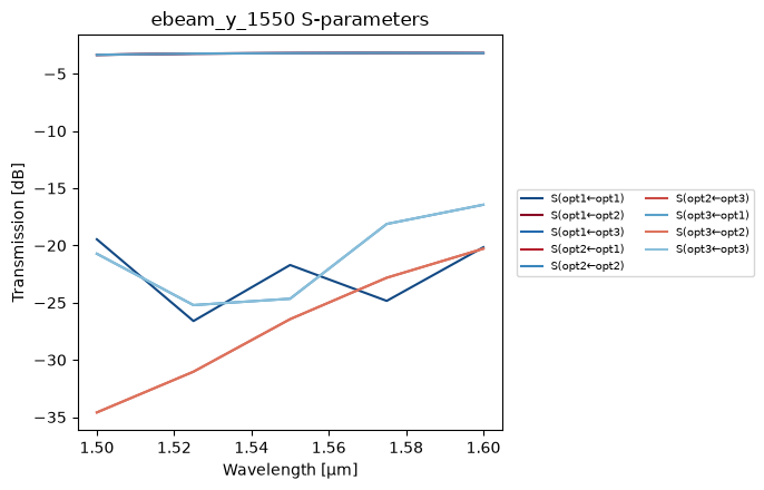
plot_smatrix overlays every measured path in dB (|S|²). A y-branch splits its input evenly, so the two transmission paths sit near −3 dB and the reflection sits far below.

plot_smatrix(sm, kind="db")
plt.show()

../_images/17dd042c0c58ec45bcd0b2ffbd5afbabf7298df3db27564c347ebae255f6ef99.png

3 · Figures of merit¶

smatrix_summary reduces the matrix to the numbers you quote in a report — insertion/return loss per path at band center, plus the physical checks.

summary = smatrix_summary(sm)
print(f"at {summary['wavelength_um']} µm:  reciprocal={summary['reciprocal']}  "
      f"passive={summary['passive']}  max power imbalance={summary['max_power_imbalance']}")
for p in summary["paths"]:
    kind = "insertion loss" if p["kind"] == "transmission" else "return loss"
    print(f"  {p['in']} → {p['out']}: {p['db']:+.2f} dB   ({kind})")

at 1.55 µm:  reciprocal=True  passive=True  max power imbalance=0.9663
  opt1 → opt2: -3.20 dB   (insertion loss)
  opt1 → opt3: -3.20 dB   (insertion loss)
  opt1 → opt1: -21.71 dB   (return loss)
  opt2 → opt1: -3.21 dB   (insertion loss)
  opt2 → opt2: -24.66 dB   (return loss)
  opt2 → opt3: -26.44 dB   (insertion loss)
  opt3 → opt1: -3.21 dB   (insertion loss)
  opt3 → opt3: -24.66 dB   (return loss)
  opt3 → opt2: -26.44 dB   (insertion loss)

4 · Phase¶

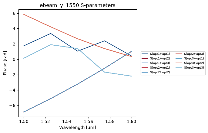
Transmission is complex — the phase (and its slope, the group delay) matters for interferometers and delay lines. kind="phase" unwraps it.

plot_smatrix(sm, kind="phase")
plt.show()

../_images/21a0971e4ba84b1132ff277e54986e719fba1ff0c4aa9d57a2f03e2b3219e633.png

5 · Physical sanity checks¶

A passive, reciprocal device must obey S = Sᵀ and inject no energy. These are your first line of defence against a mis-set simulation. Use an engineering tolerance — real FDTD output carries ~1e-3 numerical asymmetry, so a strict atol=1e-6 would flag a physically-reciprocal device as not.

print("reciprocal (S = Sᵀ):", sm.is_reciprocal(atol=1e-2))
print("passive (no gain):  ", sm.is_passive(atol=1e-2))
pb = sm.power_balance()  # 1 - Σ|S|² per input, per wavelength (loss fraction)
print(f"power balance (loss fraction) over the band: {pb.min():.3f} … {pb.max():.3f}")

reciprocal (S = Sᵀ): True
passive (no gain):   True
power balance (loss fraction) over the band: 0.471 … 0.966

Recap & next¶

The SMatrix is the common object across the toolbox: sel a path, read loss and phase, check reciprocity/passivity, and export to any standard format, the same regardless of which engine produced it.

05_fields_and_modes — the spatial picture behind these numbers.
06_convergence_and_caching — are the numbers converged?
07_choosing_an_engine — do the engines agree on them?

04 · Reading results — everything an SMatrix tells you¶