03 · Your first simulation

We’ll take a y-branch — a 1×2 power splitter — from a GDS layout all the way to S-parameters and a field profile, running on beamz: a free, open-source (Apache-2.0) FDTD engine on your own CPU. No cloud, no license.

Every simulation in gds_fdtd has the same shape:

a Component + a Technology + a SimulationSpec → one SMatrix.

Everything before run() — loading geometry, solving the waveguide mode, meshing, estimating cost — is offline and free. By the end you’ll have produced, from scratch: the material stack, the guided mode you’re launching, the meshed permittivity, the scattering matrix, and the field splitting one input into two.

from pathlib import Path

import matplotlib.pyplot as plt
import numpy as np

from gds_fdtd.grid import resolve_index
from gds_fdtd.modes import waveguide_mode
from gds_fdtd.plotting import (
    plot_component,
    plot_mode,
    plot_permittivity,
    plot_smatrix,
    plot_tech_stack,
)
from gds_fdtd.smatrix import SMatrix
from gds_fdtd.solvers import get_solver
from gds_fdtd.spec import SimulationSpec
from gds_fdtd.technology import Technology


def _find(rel: str) -> Path:
    for base in (Path.cwd(), *Path.cwd().parents):
        if (base / rel).exists():
            return base / rel
    raise FileNotFoundError(rel)


HERE = _find("examples/03_first_simulation")
tech = Technology.from_yaml(_find("examples/tech.yaml"))

1 · The device

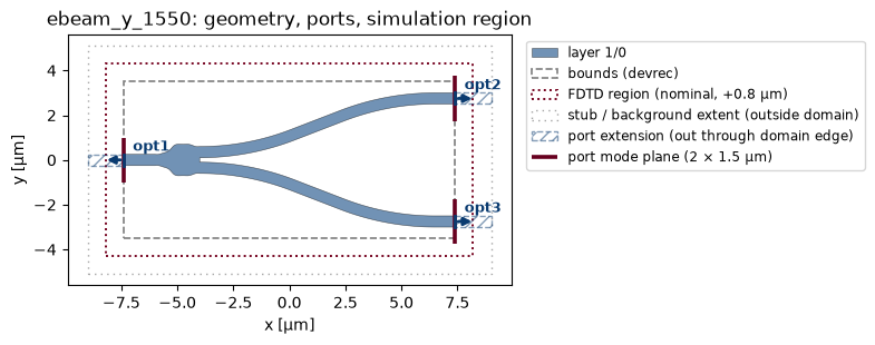
The canonical SiEPIC EBeam ebeam_y_1550 y-branch, loaded from the KLayout/SiEPIC PDK. One input (opt1, facing −x) splits into two outputs (opt2, opt3, facing +x). from_tech reads the polygons on each technology layer and auto-detects the ports — you never place them by hand.

import os  # noqa: E402

import siepic_ebeam_pdk as pdk  # noqa: E402

from gds_fdtd.lyprocessor import load_cell  # noqa: E402
from gds_fdtd.simprocessor import load_component_from_tech  # noqa: E402

gds = os.path.join(os.path.dirname(pdk.__file__), "gds", "EBeam", "ebeam_y_1550.gds")
cell, _layout = load_cell(gds, top_cell="ebeam_y_1550")
component = load_component_from_tech(cell=cell, tech=tech)
component.name = "ebeam_y_1550"

for p in component.ports:
    print(f"  {p.name}: at ({p.center[0]:.2f}, {p.center[1]:.2f}) µm, {p.width:.3f} µm wide, {p.direction}°")

plot_component(component, spec=SimulationSpec(buffer=0.8))
plt.show()

SiEPIC-EBeam-PDK Python module: siepic_ebeam_pdk, KLayout technology: EBeam
KLayout SiEPIC-Tools version 0.5.31
SiEPIC-Tools is up to date (0.5.31 vs 0.5.31).
Version check, time: 0.2743494510650635 seconds
SiEPIC-EBeam-PDK Python module: pymacros, v0.4.53
Libraries associated with Technology EBeam: ['EBeam', 'EBeam-ANT', 'EBeam-Dream', 'EBeam-SiN', 'EBeam_Beta']
  opt1: at (-7.40, 0.00) µm, 0.500 µm wide, 180°
  opt2: at (7.40, 2.75) µm, 0.500 µm wide, 0°
  opt3: at (7.40, -2.75) µm, 0.500 µm wide, 0°

19:01:42 PDT WARNING: Using canonical configuration directory at                
             '/home/mustafa/.config/tidy3d'. Found legacy directory at          
             '~/.tidy3d', which will be ignored. Remove it manually or run      
             'tidy3d config migrate --delete-legacy' to clean up.               

2 · The material stack

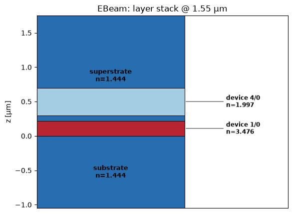
The vertical make-up of the chip: a silicon (n ≈ 3.48) waveguide core on an oxide substrate, clad in more oxide (n ≈ 1.44). This one technology file feeds every engine.

plot_tech_stack(tech, wavelength_um=1.55)
plt.show()

3 · The mode we’re launching

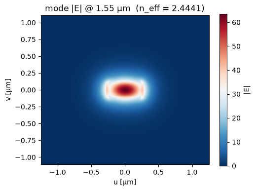
Before any light propagates, what guided mode does the input waveguide carry? We solve it locally (tidy3d’s offline mode solver — no cloud) for the strip’s actual width and thickness. Its effective index n_eff is the single number that says how the mode travels; the profile shows the light hugging the high-index core.

n_core = resolve_index(tech.device[0].material, 1.55).real
n_clad = resolve_index(tech.superstrate.material, 1.55).real
width = component.ports[0].width  # the input strip width
height = tech.device[0].z_span  # core thickness

mode = waveguide_mode(width, height, n_core, n_clad, 1.55)[0]
print(f"input strip {width:.3f}×{height:.3f} µm — TE0 n_eff = {mode.n_eff.real:.4f}")
plot_mode(mode)
plt.show()

19:01:43 PDT WARNING: Use the remote mode solver with subpixel averaging for    
             better accuracy through 'tidy3d.web.run(...)' or the deprecated    
             'tidy3d.plugins.mode.web.run(...)'. Alternatively, you can install 
             the package 'tidy3d-extras' using 'pip install "tidy3d"' and set   
             'config.simulation.use_local_subpixel=True'.                       

             WARNING: Permittivity spatial data array does not fully cover the  
             requested region.                                                  

input strip 0.500×0.220 µm — TE0 n_eff = 2.4441

4 · What the solver meshes

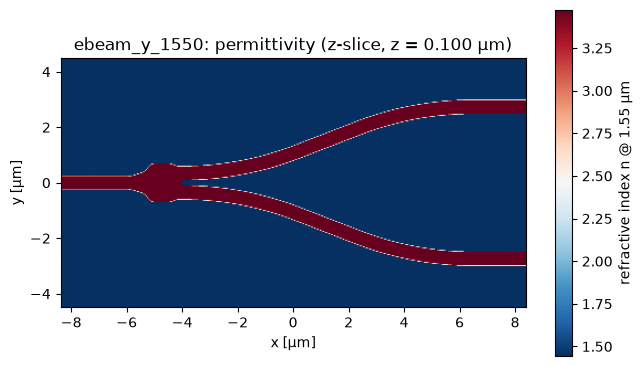
The permittivity grid the FDTD run is built on. This is the check that catches the most mistakes: whether the meshed structure is the one you intended. Here, top-down through the device layer, the input taper fans out into the two branches.

plot_permittivity(component, dx=0.04, axis="z")
plt.show()

5 · A free preview

validate() lists any problems (empty = good). build() constructs the full scene offline; estimate() reports the grid size and cost before you spend anything. We keep the job small (mesh 6, five wavelengths) so it fits a modest laptop.

spec = SimulationSpec(
    wavelength_start=1.5, wavelength_end=1.6, wavelength_points=5, mesh=6,
    z_min=-1.0, z_max=1.11, buffer=0.8,
)
solver = get_solver("beamz")(component, technology=tech, spec=spec)
print("validate():", solver.validate() or "OK — no problems")
print("build():   ", solver.build().summary)
print("estimate():", solver.estimate())

validate(): OK — no problems
● Done: Raster cache hit (3d): dca6d737c3723a585c9eb01d32dd50db74e0714717c236888fc1201314872189.npz | load=0.30s
build():    {'n_ports': 3, 'grid_shape': (70, 161, 279), 'dx_nm': 74.31914077483697, 'n_core': 3.476, 'n_clad': 1.444, 'n_simulations': 3}
estimate(): ResourceEstimate(grid_cells=3144330, memory_gb=0.15092784, n_simulations=3, cost_hint='free local compute (JAX; CPU works, GPU if available)')

6 · Run

run() is the one call that consumes a resource — on beamz, local CPU time (a few minutes) at zero cost. It returns the canonical SMatrix. We ran it once and saved the result, so this notebook re-executes instantly:

smatrix = solver.run_cached(".gds_fdtd_cache")   # repeats are free

smatrix = SMatrix.from_npz(str(_find("examples/07_choosing_an_engine/recorded/ybranch_beamz.npz")))

# a y-branch's figure of merit is its input split: opt1 into each arm
s21 = float(np.mean(smatrix.magnitude_db(out=2, in_=1)))
s31 = float(np.mean(smatrix.magnitude_db(out=3, in_=1)))
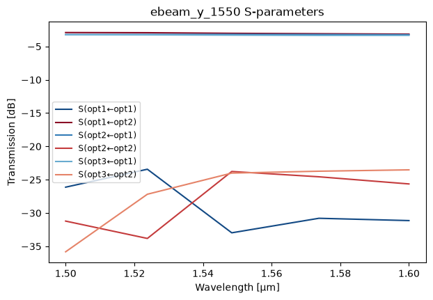
print(f"input split — opt2←opt1: {s21:.2f} dB   opt3←opt1: {s31:.2f} dB")
print("(an ideal lossless 1×2 splitter gives −3.01 dB into each arm)")

input split — opt2←opt1: -3.21 dB   opt3←opt1: -3.29 dB
(an ideal lossless 1×2 splitter gives −3.01 dB into each arm)

Power from opt1 divides roughly in half into the two arms, within a few tenths of a dB of the −3 dB ideal. The plot shows how that split holds across the wavelength band.

plot_smatrix(smatrix, kind="db")
plt.show()

7 · The field

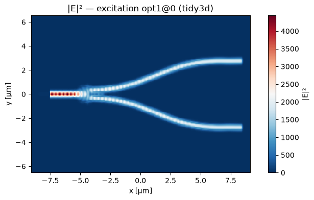
The |E|² intensity in the device plane for the opt1 excitation. The mode launched into the single input waveguide tapers out and splits evenly down the two branches.

(This field was rendered from a small tidy3d cloud run of the same y-branch — the compute is remote, so a full 3-D field costs no local memory. Every engine can produce this; 07_choosing_an_engine compares all three.)

fld = np.load(HERE / "recorded" / "ybranch_tidy3d_field.npz")
mag2 = fld["mag2"]  # (nx, ny) |E|² at band center, opt1 excitation
fig, ax = plt.subplots(figsize=(9, 4))
# tidy3d's adaptive mesh is NON-uniform, so draw the field on its true grid
# coordinates (pcolormesh) — an imshow with a uniform extent would stretch the
# finely-meshed waveguide core and misrepresent its width.
im = ax.pcolormesh(fld["x"], fld["y"], mag2.T, shading="nearest", cmap="RdBu_r")
ax.set_aspect("equal")
fig.colorbar(im, ax=ax, label="|E|²")
ax.set_xlabel("x [µm]")
ax.set_ylabel("y [µm]")
ax.set_title(f"|E|² — excitation {str(fld['source'])} (tidy3d)")
plt.show()

Recap & where to go next

From a GDS file you produced a full FDTD result — geometry, the launched mode, the mesh, a scattering matrix, and the field — with one free engine and no hand-tuning. The same five lines drive tidy3d and Lumerical too.

• 04_reading_results — everything an SMatrix can tell you (loss, crosstalk, phase, reciprocity/passivity, and I/O to Touchstone/HDF5).

• 05_fields_and_modes — higher-order modes, dispersion of n_eff, and richer field views.

• 07_choosing_an_engine — this very y-branch on beamz, tidy3d, and Lumerical, and how closely they agree.