06 · Convergence, caching, and cross-validation

Three questions decide whether you can trust an FDTD number:

1. How fine a mesh do I need? — convergence.sweep reruns a job while stepping the mesh and measures how much the S-matrix still moves.

2. How do I avoid paying for the same run twice? — run_cached hashes the whole job and reloads the stored result on a repeat.

3. Is my converged answer correct? A sweep tells you when an engine has stopped changing, which is not the same as stopping at the right value. To check that, cross-check a second engine.

§1–2 run on free beamz (a straight waveguide). §3 tackles question 3 on a hard device using recorded beamz + tidy3d + Lumerical results, so the whole notebook reproduces for free — no cloud account or license needed. §4 replays the BeamZ 0.5.3 / RTX 3090 S-bend study from committed JSON; the large mesh-30 simulations are not rerun by this notebook.

Updated result (2026-10-04): the final two through-path refinements pass 0.05 dB (0.02655 and 0.03720 dB). Mesh-30 monitor spread is 0.01371 dB at 1.55 µm. Reflections do not meet the same convergence tolerance.

Run from a repository checkout with gds_fdtd[beamz,gdsfactory] installed. Sections 1–2 execute a small local straight-waveguide sweep; sections 3–4 use recorded data. No cloud credits or licensed solvers are used.

import io
import json
import sys
import tempfile
from contextlib import redirect_stdout
from pathlib import Path

import gdsfactory as gf
import matplotlib.pyplot as plt
import numpy as np
from IPython.display import Markdown, display

from gds_fdtd.convergence import sweep
from gds_fdtd.layout.gdsfactory import from_gdsfactory
from gds_fdtd.lyprocessor import load_cell
from gds_fdtd.plotting import plot_component, plot_permittivity
from gds_fdtd.simprocessor import load_component_from_tech
from gds_fdtd.solvers import get_solver
from gds_fdtd.spec import SimulationSpec
from gds_fdtd.technology import Technology


def _find(rel: str) -> Path:
    for base in (Path.cwd(), *Path.cwd().parents):
        if (base / rel).exists():
            return base / rel
    raise FileNotFoundError(rel)


REC = _find("examples/06_convergence_and_caching/recorded")
tech = Technology.from_yaml(_find("examples/tech.yaml"))

1 · How fine a mesh? — a convergence sweep

A short straight waveguide, swept over three mesh densities on beamz. sweep returns a ConvergenceReport; max |ΔS| is the worst-case change, between successive meshes, of any S-parameter carrying real power (floor_db=-10 keeps the metric on the through path, not the deep numerical reflection of a well-matched straight). A cache_dir means only genuinely new points ever cost a run.

gf.gpdk.PDK.activate()
straight = from_gdsfactory(gf.components.straight(length=1.5), tech)
spec = SimulationSpec(
    wavelength_start=1.5, wavelength_end=1.6, wavelength_points=3, z_min=-0.6, z_max=0.8
)
cache = Path(tempfile.mkdtemp(prefix="gdsfdtd_conv_"))
mesh_values = [4, 6, 8]
TOL_DB = 0.25  # engineering tolerance — convergence is always relative to it

# Keep solver runtime diagnostics out of the displayed benchmark results.
with redirect_stdout(io.StringIO()):
    report = sweep(
        get_solver("beamz"),
        straight,
        tech,
        spec,
        field="mesh",
        values=mesh_values,
        cache_dir=cache,
        floor_db=-10.0,
    )

for lo, hi, d in zip(mesh_values, mesh_values[1:], report.deltas_db, strict=False):
    print(f"mesh {lo} → {hi}:  max |ΔS| = {d:.3f} dB")
rec = report.recommend(tol_db=TOL_DB)
print(f"\nfirst candidate mesh at tolerance {TOL_DB} dB: {rec}")

mesh 4 → 6:  max |ΔS| = 0.218 dB
mesh 6 → 8:  max |ΔS| = 0.091 dB

first candidate mesh at tolerance 0.25 dB: 6

report.plot(tol_db=TOL_DB)
plt.show()

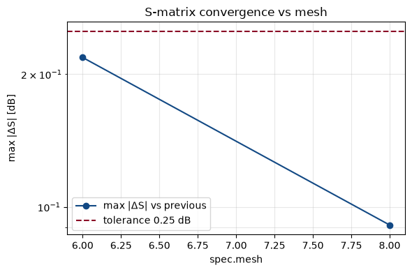
recommend returns the first swept mesh whose change from the preceding mesh is below the chosen tolerance, or None if none passes. That is a candidate resolution, not proof of an asymptotic solution or a bound on physical error. Check further refinements before making stronger claims. Section 4 requires two final refinement steps below 0.05 dB.

2 · Repeats are free — caching

Every point above was stored under a content hash. Re-running the identical sweep recomputes nothing; change the geometry, technology, spec, or engine version and only the genuinely new work reruns.

again = sweep(
    get_solver("beamz"),
    straight,
    tech,
    spec,
    field="mesh",
    values=mesh_values,
    cache_dir=cache,
    floor_db=-10.0,
)
print(f"identical result: {again.recommend(TOL_DB) == rec}")

identical result: True

3 · Historical baseline: BeamZ 0.4.3 on a hard device

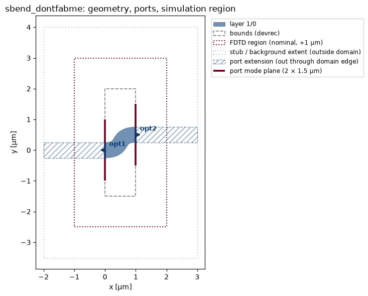
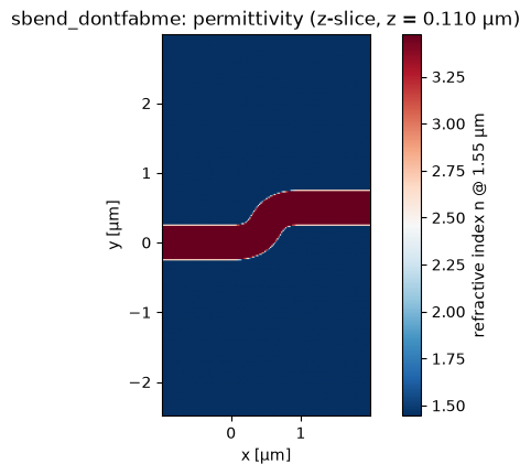
A sweep only tells you an engine stopped changing. On a benign device that’s not sufficient for accuracy; cross-check an independent reference as well. The BeamZ data in this section are 0.4.3 recordings, not the current adapter. Section 4 shows the new 0.5.3 study and its qualified conclusions. sbend_dontfabme (from examples/devices.gds) is a sharp S-bend that offsets the guide 0.5 µm in ~1 µm. A bend that tight strongly converts the fundamental mode into higher-order modes and radiation, so its true loss is large and it stresses any solver.

First, the geometry the solvers build — device + cladding + the port extensions that carry each port out through the domain edge:

sbend_cell, _ = load_cell(str(_find("examples/devices.gds")), top_cell="sbend_dontfabme")
sbend = load_component_from_tech(cell=sbend_cell, tech=tech)
sbend.name = "sbend_dontfabme"
plot_component(sbend, spec=SimulationSpec())
plt.show()
plot_permittivity(sbend, axis="z", position=0.11, wavelength_um=1.55)  # top-down √ε at the Si core
plt.show()

Historical convergence curves — BeamZ 0.4.3 vs the references

Single wavelength (1.55 µm), swept from low to high mesh on all three engines (recorded in recorded/; beamz on CPU, tidy3d on the cloud, Lumerical on a licensed workstation — its mesh maps to the nearest of Lumerical’s discrete mesh accuracy settings 1–5). S21 on the left axis, S11 on the right.

beamz_c = json.loads((REC / "sbend_beamz_convergence.json").read_text())["mesh"]
tidy3d_c = json.loads((REC / "sbend_tidy3d_convergence.json").read_text())["mesh"]
lum_c = json.loads((REC / "sbend_lumerical_convergence.json").read_text())["mesh"]

fig, axL = plt.subplots(figsize=(8, 5))
axR = axL.twinx()
bm = sorted(int(m) for m in beamz_c)
tm = sorted(int(m) for m in tidy3d_c)
lm = sorted(int(m) for m in lum_c)
axL.plot(
    bm, [beamz_c[str(m)]["s21_db"] for m in bm], "o-", color="tab:blue", label="BeamZ 0.4.3 S21"
)
axL.plot(tm, [tidy3d_c[str(m)]["s21_db"] for m in tm], "s--", color="tab:red", label="tidy3d S21")
axL.plot(lm, [lum_c[str(m)]["s21_db"] for m in lm], "^:", color="tab:green", label="Lumerical S21")
axR.plot(
    bm,
    [beamz_c[str(m)]["s11_db"] for m in bm],
    "o-",
    color="tab:blue",
    alpha=0.4,
    markerfacecolor="none",
    label="BeamZ 0.4.3 S11",
)
axR.plot(
    tm,
    [tidy3d_c[str(m)]["s11_db"] for m in tm],
    "s--",
    color="tab:red",
    alpha=0.4,
    markerfacecolor="none",
    label="tidy3d S11",
)
axR.plot(
    lm,
    [lum_c[str(m)]["s11_db"] for m in lm],
    "^:",
    color="tab:green",
    alpha=0.4,
    markerfacecolor="none",
    label="Lumerical S11",
)
axL.set_xlabel("mesh setting (engine-specific)")
axL.set_ylabel("S21  |through|  [dB]")
axR.set_ylabel("S11  |reflection|  [dB]")
axL.set_title("Historical S-bend at 1.55 µm — BeamZ 0.4.3 vs recorded references")
axL.grid(True, alpha=0.3)
_ln = axL.get_lines() + axR.get_lines()
axL.legend(_ln, [ln.get_label() for ln in _ln], loc="center right", fontsize=8)
fig.tight_layout()
plt.show()

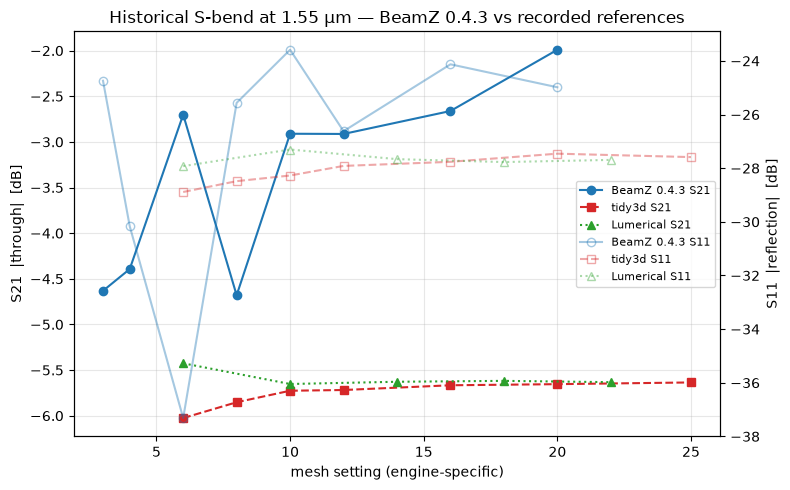
The recorded Tidy3D and Lumerical through-path curves approach about −5.63 dB. BeamZ 0.4.3 did not converge toward those references in this sweep: its mesh-20 value was −1.99 dB. This historical result motivated the integration and modal-analysis investigation. It does not imply that newer BeamZ versions fail in the same way; see the 0.5.3 evidence in §4. Agreement between references supports the comparison, but is not an exact ground truth when discretization, materials, and port definitions differ.

Historical launched-mode comparison

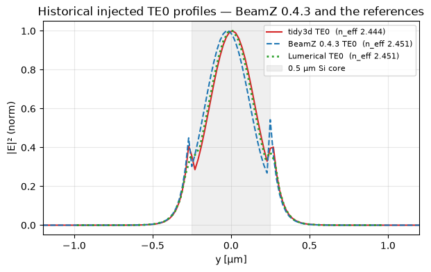
A wider field could mean a different injected mode. It does not: all three mode solvers — tidy3d’s local plugin, beamz’s, and Lumerical’s port FDE (extracted from the port that feeds its FDTD run) — find the fundamental TE0 of the 0.5 µm guide at nearly identical effective index, and their lateral profiles sit on top of each other. The waveguide and the launched mode are the same across engines, so whatever differs downstream is not a wider guide.

md = np.load(REC / "sbend_injected_modes.npz")
fig, ax = plt.subplots(figsize=(7, 4))
ax.plot(
    md["y_tidy3d"],
    md["e2_tidy3d"],
    color="tab:red",
    label=f"tidy3d TE0  (n_eff {float(md['neff_tidy3d']):.3f})",
)
ax.plot(
    md["y_beamz"],
    md["e2_beamz"],
    "--",
    color="tab:blue",
    label=f"BeamZ 0.4.3 TE0  (n_eff {float(md['neff_beamz']):.3f})",
)
ax.plot(
    md["y_lumerical"],
    md["e2_lumerical"],
    ":",
    color="tab:green",
    lw=2,
    label=f"Lumerical TE0  (n_eff {float(md['neff_lumerical']):.3f})",
)
ax.axvspan(-0.25, 0.25, alpha=0.12, color="gray", label="0.5 µm Si core")
ax.set_xlim(-1.2, 1.2)
ax.set_xlabel("y [µm]")
ax.set_ylabel("|E|² (norm)")
ax.set_title("Historical injected TE0 profiles — BeamZ 0.4.3 and the references")
ax.grid(alpha=0.3)
ax.legend(fontsize=8)
plt.show()

Historical fields through the bend — linear and log

The panels below show how the field evolves through the bend. Top row is a linear scale (only the strong guided field shows; faint radiation can’t inflate it); bottom is log (dB) (the radiation becomes visible). Each panel is normalized to its own peak; cyan rings mark the two ports.

Rendering note. tidy3d’s adaptive mesh is non-uniform (35–90 nm cells here), so its field must be drawn on its true grid coordinates (pcolormesh); an imshow with a uniform extent stretches the finely-meshed core about 2× and makes the waveguide look wider than it is. beamz’s grid is uniform, so either rendering is faithful for it.

bz = np.load(REC / "sbend_beamz_field.npz")
t3 = np.load(REC / "sbend_tidy3d_field.npz")
lu = np.load(REC / "sbend_lumerical_field.npz")
bw, bh = float(bz["width_um"]), float(bz["height_um"])
cx, cy = sbend.bounds.x_center, sbend.bounds.y_center  # beamz's 0-based frame -> device coords
# beamz: uniform grid -> cell-center coordinate vectors in device µm
b_x = np.linspace(cx - bw / 2, cx + bw / 2, bz["E2"].shape[1])
b_y = np.linspace(cy - bh / 2, cy + bh / 2, bz["E2"].shape[0])
# tidy3d + Lumerical: their own (possibly non-uniform) grid coordinates
panels = [
    ("BeamZ 0.4.3", b_x, b_y, bz["E2"], float(bz["s21"])),
    ("tidy3d", t3["x"], t3["y"], t3["E2"].T, float(t3["s21"])),
    ("Lumerical", lu["x"], lu["y"], lu["E2"].T, float(lu["s21"])),
]

fig, ax = plt.subplots(2, 3, figsize=(16.5, 9.5), constrained_layout=True)
for col, (name, gx, gy, e2, s21) in enumerate(panels):
    en = e2 / e2.max()
    im_lin = ax[0, col].pcolormesh(gx, gy, en, shading="nearest", cmap="magma", vmin=0, vmax=1)
    ax[0, col].set_title(f"{name}  linear   (S21 = {s21:+.2f} dB)")
    im_log = ax[1, col].pcolormesh(
        gx,
        gy,
        10 * np.log10(np.clip(en, 1e-4, 1)),
        shading="nearest",
        cmap="magma",
        vmin=-40,
        vmax=0,
    )
    ax[1, col].set_title(f"{name}  log [dB]")
    for r in (0, 1):
        ax[r, col].scatter([0, 1], [0, 0.5], s=36, edgecolor="cyan", facecolor="none", lw=1.5)
        ax[r, col].set_xlim(cx - 1.9, cx + 1.9)
        ax[r, col].set_ylim(cy - 2, cy + 2)
        ax[r, col].set_aspect("equal")
        ax[r, col].set_xlabel("x [µm]")
        ax[r, col].set_ylabel("y [µm]")
fig.colorbar(im_lin, ax=ax[0, :], label="|E|² (norm)", shrink=0.7)
fig.colorbar(im_log, ax=ax[1, :], label="|E|² [dB]", shrink=0.7)
fig.suptitle("Historical z-plane |E|² — BeamZ 0.4.3 and recorded commercial references")
plt.show()

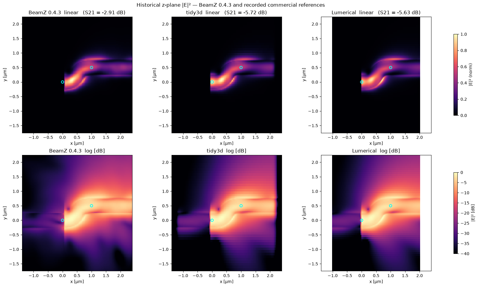
The historical field maps look broadly comparable, while their extracted modal transmission differs substantially. A field image alone cannot validate an S-parameter. The comparisons also retain engine-specific grid, material, sidewall, and reference-plane differences.

The old data demonstrate a discrepancy; they do not by themselves establish a unique root cause. The current adapter and BeamZ 0.5.3 use a different extraction path, including the material-snapshot correction for issue #309.

4 · Updated study: BeamZ 0.5.3 on the RTX 3090

This section loads the completed mesh 10/14/20/25/30 sweep. No simulation runs here. Geometry, materials, domain, source/monitor positions, and all non-mesh settings are fixed. Only resolution and its associated time step change. The mesh-30 runs use JAX’s platform allocator to fit GPU memory; the device run logged an allocation warning, then completed successfully.

The declared criterion is both final successive through-path changes below 0.05 dB, worst case across both transmission directions and all three samples (1.600000, 1.548387, 1.500000 µm), with floor_db=-10. This is a successive-change tolerance, not an absolute-error bound.

Sources: study report, JSON measurements, and execution notes. The 1.55 µm values below are interpolated in frequency in dB.

repo_root = _find("pyproject.toml").parent
benchmark_dir = repo_root / "benchmarks"
if str(benchmark_dir) not in sys.path:
    sys.path.insert(0, str(benchmark_dir))
from beamz_mesh_convergence import magnitude_delta  # noqa: E402
from compare_beamz_devices import db_at  # noqa: E402
from magnitude_results import MagnitudeResults  # noqa: E402

study_dir = benchmark_dir / "results/beamz-0.5.3-convergence"
study = json.loads((study_dir / "summary.json").read_text())
mesh_values_053 = [row["mesh"] for row in study["runs"]]
assert mesh_values_053 == [10, 14, 20, 25, 30]
records = []
for mesh in mesh_values_053:
    folder = benchmark_dir / "results/beamz-0.5.3-validation" if mesh in (10, 20) else study_dir
    records.append(MagnitudeResults(folder / f"sbend-mesh{mesh}/results.json"))
for matrix in records:
    assert matrix.record["beamz"] == "0.5.3"
    assert matrix.record["finite"]
    assert all(run["termination"]["converged"] for run in matrix.record["runs"])
    assert all(
        source["all_incident_samples_valid"] for source in matrix.record["modal_sources"].values()
    )
    assert matrix.record["gds_sha256"] == records[0].record["gds_sha256"]
    assert matrix.record["ports"] == records[0].record["ports"]
    assert {k: v for k, v in matrix.record["spec"].items() if k != "mesh"} == {
        k: v for k, v in records[0].record["spec"].items() if k != "mesh"
    }
    for key in ("diagnostic_monitor_offset_um", "diagnostic_source_offset_um"):
        assert matrix.record[key] == records[0].record[key]
    np.testing.assert_array_equal(matrix.wavelength_um, records[0].wavelength_um)
through_deltas = [
    magnitude_delta(a, b, -10) for a, b in zip(records[:-1], records[1:], strict=True)
]
all_entry_deltas = [
    magnitude_delta(a, b, -40) for a, b in zip(records[:-1], records[1:], strict=True)
]
np.testing.assert_allclose(
    through_deltas,
    [r["through_max_delta_db"] for r in study["successive_deltas"]],
    atol=1e-10,
    rtol=0,
)
np.testing.assert_allclose(
    all_entry_deltas,
    [r["matrix_max_delta_db_floor_minus40"] for r in study["successive_deltas"]],
    atol=1e-10,
    rtol=0,
)
through_pass = all(value < study["tolerance_db"] for value in through_deltas[-2:])
assert through_pass == study["mesh_criterion_passed"]
print("Loaded and checked five fixed-setup BeamZ 0.5.3 runs; all source/stopping checks pass.")

Loaded and checked five fixed-setup BeamZ 0.5.3 runs; all source/stopping checks pass.

Transmission, reflection, and the declared tolerance

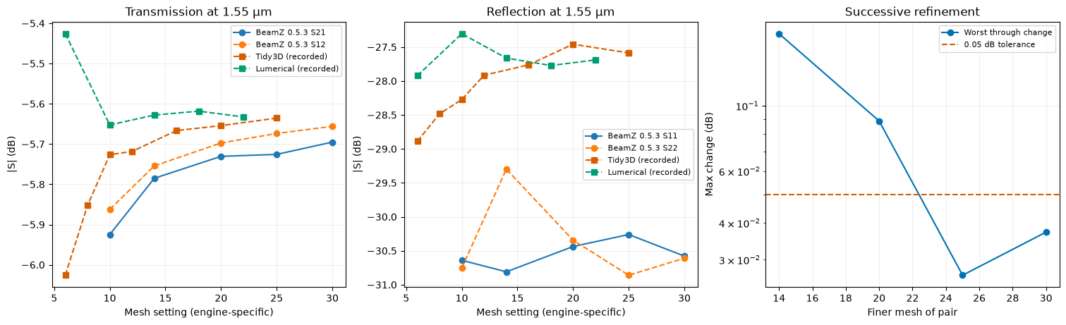
Recompute the values from per-run JSON magnitudes, rather than copying a rendered image. Both directions are included in the successive-change test. The separate reflection panel prevents a through-path pass from being mistaken for full-matrix convergence.

fig, axes = plt.subplots(1, 3, figsize=(15, 4.5), layout="constrained")
for out, source, style, label in [
    (2, 1, "o-", "BeamZ 0.5.3 S21"),
    (1, 2, "o--", "BeamZ 0.5.3 S12"),
]:
    axes[0].plot(mesh_values_053, [db_at(m, out, source) for m in records], style, label=label)
for port, style in [(1, "o-"), (2, "o--")]:
    axes[1].plot(
        mesh_values_053,
        [db_at(m, port, port) for m in records],
        style,
        label=f"BeamZ 0.5.3 S{port}{port}",
    )
for engine, values, color in [("Tidy3D", tidy3d_c, "#D55E00"), ("Lumerical", lum_c, "#009E73")]:
    meshes = sorted(map(int, values))
    for ax, key in [(axes[0], "s21_db"), (axes[1], "s11_db")]:
        ax.plot(
            meshes,
            [values[str(m)][key] for m in meshes],
            "s--",
            color=color,
            label=f"{engine} (recorded)",
        )
for ax, title in zip(axes[:2], ["Transmission at 1.55 µm", "Reflection at 1.55 µm"], strict=True):
    ax.set(title=title, xlabel="Mesh setting (engine-specific)", ylabel="|S| (dB)")
axes[2].semilogy(
    mesh_values_053[1:], through_deltas, "o-", color="#0072B2", label="Worst through change"
)
axes[2].axhline(study["tolerance_db"], color="#D55E00", linestyle="--", label="0.05 dB tolerance")
axes[2].set(title="Successive refinement", xlabel="Finer mesh of pair", ylabel="Max change (dB)")
for ax in axes:
    ax.grid(alpha=0.2)
    ax.legend(fontsize=8)
plt.show()

rows = [
    "| Refinement | Through change (dB) | All-entry change, −40 dB floor | Through pass? |",
    "|---|---:|---:|---|",
]
for lo, hi, delta, full_delta in zip(
    mesh_values_053[:-1], mesh_values_053[1:], through_deltas, all_entry_deltas, strict=True
):
    rows.append(
        f"| {lo} → {hi} | {delta:.5f} | {full_delta:.5f} | "
        f"{'Yes' if delta < study['tolerance_db'] else 'No'} |"
    )
display(Markdown("\n".join(rows)))
display(
    Markdown(
        f"**Final two through refinements: {'PASS' if through_pass else 'FAIL'}.** "
        f"Mesh-30 S21 = **{db_at(records[-1], 2, 1):.5f} dB** at 1.55 µm."
    )
)

| Refinement | Through change (dB) | All-entry change, −40 dB floor | Through pass? | |—|—:|—:|—| | 10 → 14 | 0.17567 | 2.48032 | No | | 14 → 20 | 0.08872 | 1.05972 | No | | 20 → 25 | 0.02655 | 0.53283 | Yes | | 25 → 30 | 0.03720 | 0.50777 | Yes |

Final two through refinements: PASS. Mesh-30 S21 = -5.69511 dB at 1.55 µm.

The final through changes are 0.02655 and 0.03720 dB, both below 0.05 dB. The latter increases slightly: this is not a proof of monotonic or asymptotic error decay. The final all-entry change is 0.50777 dB, dominated by reflections; the full matrix does not pass the same tolerance.

Default-plane S21 at mesh 30 is −5.69511 dB, about 0.06 dB from the finest recorded commercial references. Successive-grid stability and agreement with another engine are distinct checks; neither guarantees exact physical truth.

Updated fields through the bend — BeamZ 0.5.3

The same linear/log comparison, now using the mesh-30 BeamZ 0.5.3 RTX3090 run from the convergence study. Excitation is opt1, with the horizontal slice at z = 0.11 µm and the recorded center-frequency sample at λ = 1.54839 µm. Commercial fields below are the existing 1.55 µm recordings (Tidy3D mesh 12; Lumerical ppw 14 / accuracy 3); their runs have not been repeated. These are not the finest-grid commercial references in the separate convergence curves. S21 labels use the 1.55 µm values, interpolated for BeamZ.

These maps show normalized electric-field intensity, |E|², not Poynting flux or calibrated transmitted power. Each engine is normalized to its own full-plane peak, so compare spatial patterns rather than absolute brightness. BeamZ’s native Yee components are summed without spatial collocation and shown at cell-center display coordinates. The commercial grids retain their recorded coordinates. Cyan rings mark the device ports; the white strip beyond the Lumerical recording indicates unavailable data, not zero intensity.

The portable JSON stores the displayed crop at native spatial resolution (six significant digits). It is derived from the locally retained complex field archive by benchmarks/export_beamz_field.py; the archive is not added to the repository. Provenance includes the run path and source-file hash.

field_053 = json.loads((REC / "sbend_beamz_053_intensity.json").read_text())
assert field_053["beamz"] == "0.5.3" and field_053["mesh"] == 30
assert field_053["gds_sha256"] == records[-1].record["gds_sha256"]
e2_053 = np.asarray(field_053["intensity_normalized"])
assert e2_053.shape == (len(field_053["y_um"]), len(field_053["x_um"]))
assert np.isfinite(e2_053).all() and np.all((e2_053 >= 0) & (e2_053 <= 1))
current_panels = [
    (
        "BeamZ 0.5.3 · mesh 30",
        field_053["x_um"],
        field_053["y_um"],
        e2_053,
        db_at(records[-1], 2, 1),
    ),
    ("Tidy3D · recorded", t3["x"], t3["y"], t3["E2"].T / t3["E2"].max(), float(t3["s21"])),
    ("Lumerical · recorded", lu["x"], lu["y"], lu["E2"].T / lu["E2"].max(), float(lu["s21"])),
]
fig, axes = plt.subplots(2, 3, figsize=(13, 9), layout="constrained")
for col, (name, x, y, intensity, s21) in enumerate(current_panels):
    linear = axes[0, col].pcolormesh(
        x, y, intensity, shading="nearest", cmap="magma", vmin=0, vmax=1
    )
    logarithmic = axes[1, col].pcolormesh(
        x,
        y,
        10 * np.log10(np.clip(intensity, 1e-4, 1)),
        shading="nearest",
        cmap="magma",
        vmin=-40,
        vmax=0,
    )
    axes[0, col].set_title(f"{name}\nLinear · S21 = {s21:+.2f} dB")
    axes[1, col].set_title(f"{name}\nLogarithmic")
    for ax in axes[:, col]:
        ax.scatter([0, 1], [0, 0.5], s=36, edgecolor="cyan", facecolor="none", lw=1.5)
        ax.set(
            xlim=(cx - 1.9, cx + 1.9),
            ylim=(cy - 2, cy + 2),
            xlabel="x (µm)",
            ylabel="y (µm)",
            aspect="equal",
        )
fig.colorbar(linear, ax=axes[0, :], label="|E|² / full-plane peak", shrink=0.75)
fig.colorbar(logarithmic, ax=axes[1, :], label="Normalized |E|² (dB)", shrink=0.75)
fig.suptitle("Sharp S-bend electric-field intensity · z = 0.11 µm")
plt.show()

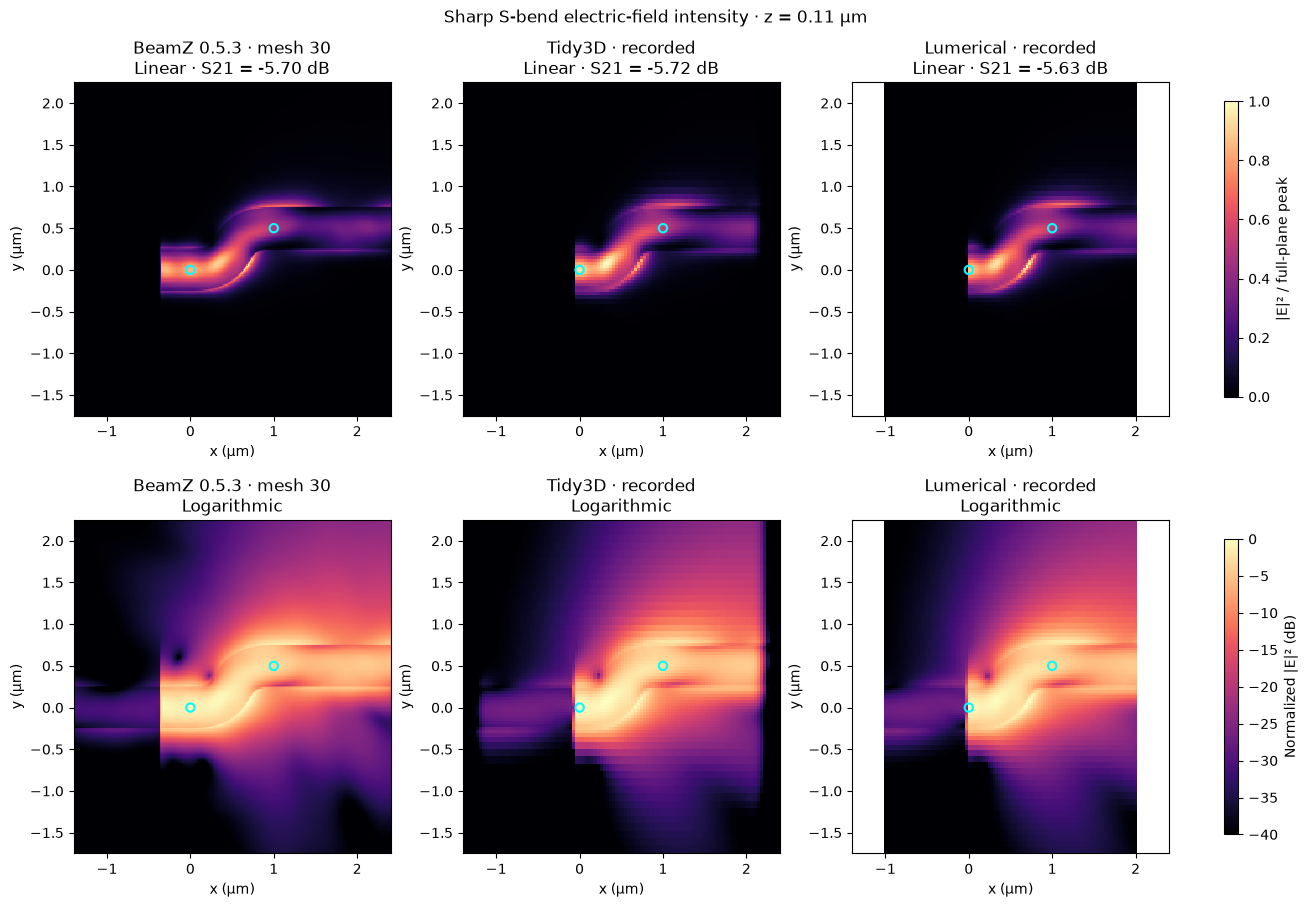
The maps provide a spatial check of the guided field and radiation through the sharp bend. Peak normalization does not establish transmission accuracy; the separate S-parameter and refinement checks above remain the quantitative evidence.

Does monitor placement still matter?

Each probe run holds the source and input monitor fixed and samples five output planes simultaneously. Positive distances lie in the straight lead. The −0.05 µm plane is inside the bend and is excluded from the lead-spread metric, but remains visible. The primary mesh sweep above retains that default inside-bend plane; a favorable plane was not substituted into it.

fig, axes = plt.subplots(1, 2, figsize=(11, 4.5), layout="constrained")
probe_spreads = []
for mesh, color in [(10, "0.5"), (20, "#56B4E9"), (30, "#0072B2")]:
    if mesh == 10:
        path = benchmark_dir / "results/beamz-0.5.3-validation/native-probe-mesh10.json"
    else:
        folder = benchmark_dir / "results/beamz-0.5.3-validation" if mesh == 20 else study_dir
        path = folder / f"sbend-plane-probe-mesh{mesh}/probe.json"
    probe = json.loads(path.read_text())
    assert probe["beamz"] == "0.5.3" and probe["termination"]["converged"]
    assert all(probe["valid_mask"])
    distance = -np.asarray(probe["output_inward_offsets_um"])
    values = np.asarray([probe["s21_db"][f"out_{i}"] for i in range(5)])
    spread = np.ptp(values[distance > 0], axis=0)
    recorded = next(p for p in study["probes"] if p["mesh"] == mesh)
    np.testing.assert_allclose(spread, recorded["lead_spread_db"], atol=1e-10, rtol=0)
    probe_spreads.append(spread)
    axes[0].plot(distance, values[:, 1], "o-", color=color, label=f"Mesh {mesh}")
axes[0].axvline(0, color="0.5", linestyle=":")
axes[0].set(
    title="Same-run probes at 1.55 µm", xlabel="Distance outward from port (µm)", ylabel="S21 (dB)"
)
for index, wavelength in enumerate(probe["wavelength_um"]):
    axes[1].plot(
        [10, 20, 30], np.asarray(probe_spreads)[:, index], "o-", label=f"{wavelength:.2f} µm"
    )
axes[1].axhline(0.05, color="0.5", linestyle="--", label="0.05 dB tolerance")
axes[1].set(title="Uniform-lead monitor spread", xlabel="Mesh", ylabel="Max − min S21 (dB)")
for ax in axes:
    ax.grid(alpha=0.2)
    ax.legend(fontsize=8)
plt.show()
assert max(probe_spreads[-1]) < study["tolerance_db"]
print(f"Mesh-30 lead spread at 1.55 µm: {probe_spreads[-1][1]:.5f} dB")
print(
    f"Mesh-30 lead spread across probe wavelengths: "
    f"{min(probe_spreads[-1]):.5f}–{max(probe_spreads[-1]):.5f} dB"
)

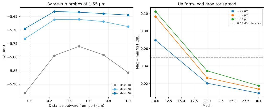
Mesh-30 lead spread at 1.55 µm: 0.01371 dB
Mesh-30 lead spread across probe wavelengths: 0.00904–0.01752 dB

At mesh 30 the straight-lead spread is 0.01371 dB at 1.55 µm and 0.00904–0.01752 dB across the three probe wavelengths. All four lead readings at 1.55 µm lie between −5.63109 and −5.64479 dB, within 0.013 dB of both recorded references. The inside-bend plane reads −5.69467 dB in the same run. These distinct locations should not be treated as interchangeable.

Recap & next

• BeamZ 0.5.3 passes the declared successive-mesh criterion for the sampled through paths of this sharp S-bend, and its finest-grid lead spread is small.

• Reflections do not pass the same tolerance. Complex phase, PML/domain convergence, other devices, TM, multimode, and y-facing ports are not validated by this study. Material and reference-plane differences remain.

• The old 0.4.3 failure is historical evidence, not a description of 0.5.3.

• sweep measures mesh changes; run_cached avoids rerunning identical jobs; independent references and monitor checks address different accuracy risks.

See the full study and reproduction commands to rerun the GPU jobs. Generated binary arrays remain local; this section uses the committed JSON measurements. Next: 07_choosing_an_engine.