Working with S-Parameters

S-parameters (scattering parameters) characterize how a photonic component routes optical power between its ports. In gds_fdtd every solver returns one canonical container (gds_fdtd.smatrix.SMatrix) regardless of the engine, so the analysis below is identical for tidy3d, Lumerical, and beamz.

S-Parameter Fundamentals

S-parameters describe how waves scatter through a multi-port network:

• S₁₁: reflection at port 1 when excited at port 1

• S₂₁: transmission from port 1 to port 2

• S₁₂: transmission from port 2 to port 1

• S₂₂: reflection at port 2 when excited at port 2

For multi-modal devices each path also carries mode indices (mode 1 = TE-like, mode 2 = TM-like), e.g. S₂₁⁽ᵀᴱ→ᵀᴹ⁾ is TE→TM conversion from port 1 to 2. See Multi-Modal Simulations for the multi-mode workflow.

Getting the S-matrix

run() is the only method that spends money/licenses/compute; it returns an SMatrix. Nothing is stored on the solver; hold onto the returned object:

from gds_fdtd.solvers import get_solver
from gds_fdtd.spec import SimulationSpec

solver = get_solver("tidy3d")(component, technology=tech, spec=SimulationSpec())
smatrix = solver.run()          # -> gds_fdtd.smatrix.SMatrix

print(f"Component:       {smatrix.name}")
print(f"Ports:           {smatrix.n_ports} {smatrix.port_names}")
print(f"Modes:           {smatrix.n_modes}")
print(f"Frequency pts:   {smatrix.f.size}")

Wavelength / frequency grids

wavelengths_um = smatrix.wavelength_um   # micrometers (descending as f ascends)
frequencies_hz = smatrix.f               # Hz, ascending

print(f"Wavelength range: {wavelengths_um.min():.3f} - {wavelengths_um.max():.3f} um")

Accessing individual paths

Ports are addressed by name ("opt1") or by their trailing-digit id (1); modes are 1-based. sel returns the complex response; magnitude_db returns |S|² in dB. Both are (F,) arrays over the wavelength grid.

import numpy as np

# complex transmission port1 -> port2 (fundamental mode)
s21 = smatrix.sel(out="opt2", in_="opt1", mode_out=1, mode_in=1)

# the same path in dB (|S|^2)
s21_db = smatrix.magnitude_db(out="opt2", in_="opt1")   # modes default to 1

# reflection at port 1
s11_db = smatrix.magnitude_db(out="opt1", in_="opt1")

print(f"Peak transmission: {s21_db.max():.2f} dB")
print(f"Peak reflection:   {s11_db.max():.2f} dB")

Unmeasured paths (partial matrices) are NaN. A device simulated with only port 1 excited leaves the port-2-excited columns NaN, which the accessors, physics checks, and exporters all handle.

Physics checks

The checks operate on the full (port, mode)-flattened matrix and are NaN-aware (only mutually measured pairs count):

smatrix.is_reciprocal()          # S == S^T within tolerance
smatrix.is_passive()             # no excitation outputs more power than it received
balance = smatrix.power_balance()  # sum_out |S|^2 per (freq, in-port*mode) excitation

For a lossless, reciprocal device power_balance() sits near 1.0 and both predicates return True (within atol).

Plotting

plot_smatrix plots every measured path versus wavelength (paths whose peak is below −60 dB are hidden so large matrices stay readable):

from gds_fdtd.plotting import plot_smatrix

fig, ax = plot_smatrix(smatrix, kind="db")     # kind: "db" | "linear" | "phase"
fig.savefig("device_sparams.png", dpi=150, bbox_inches="tight")

# restrict to specific (out, in, mode_out, mode_in) paths:
paths = [("opt2", "opt1", 1, 1), ("opt1", "opt1", 1, 1)]
plot_smatrix(smatrix, kind="db", paths=paths)

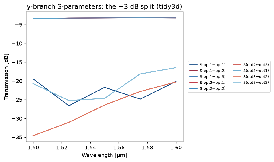
A y-branch S-matrix: the two transmission paths near −3 dB, reflection far below.

Exporting

SMatrix writes the standard interchange formats directly, no hand-rolled writers needed:

smatrix.to_dat("device.dat")          # Lumerical INTERCONNECT (partial matrices OK)
smatrix.to_touchstone("device.s2p")   # Touchstone v1 (.sNp; N = n_ports*n_modes)
smatrix.to_hdf5("device.h5")          # requires h5py
smatrix.to_npz("device.npz")          # numpy built-in, always available

# round-trips back to an SMatrix:
from gds_fdtd.smatrix import SMatrix
again = SMatrix.from_dat("device.dat")

Notes:

• .dat and .npz/.h5 preserve NaN (unmeasured) paths; Touchstone requires a complete matrix and raises on NaN, export .dat for partial matrices.

• Touchstone flattens (port, mode) pairs port-major; the ordering is written into the file header.

• .dat is round-trip lossless (to_dat → from_dat); the INTERCONNECT reader/writer is an internal helper (gds_fdtd._sparams), use the SMatrix methods above rather than importing it.

Working offline with recorded results

You do not need an engine to exercise the S-matrix API; examples/04_reading_results loads a recorded real result and gives the full offline tour of the I/O, physics checks, and plotting. For the Lumerical INTERCONNECT .dat format specifically:

from gds_fdtd.smatrix import SMatrix

sm = SMatrix.from_dat("examples/10_cookbook/recorded/si_sin_escalator.dat")
print(sm.is_reciprocal(), sm.is_passive())
plot_smatrix(sm, kind="db")

See also Multi-Modal Simulations (multi-mode / polarization) and Setting Up Simulations (the end-to-end GDS → S-parameters flow).