11 · A Bragg grating: the stopband, seen in the field

A waveguide Bragg grating is a strip whose width is corrugated with period Λ. Each corrugation reflects a sliver of the guided wave; at the Bragg wavelength λ_B = 2·n_eff·Λ the slivers add in phase and the grating turns into a mirror. Away from λ_B they cancel and the light passes as if the grating were a plain waveguide.

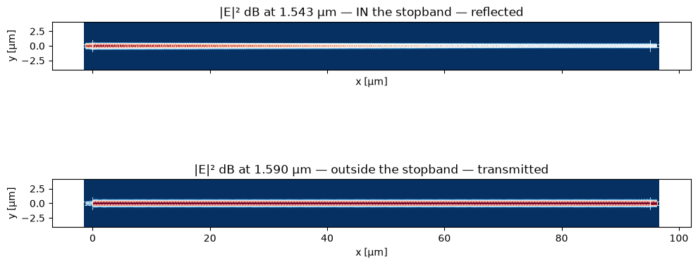
That makes a Bragg grating the perfect device to watch through a field monitor at two wavelengths: in-band the field piles up at the entrance and decays into the grating (reflected); out-of-band it sails through. Both pictures come from one simulation — the monitor records several chosen wavelengths (spec.field_monitor_wavelengths), and the plot selects among them.

The device is bragg_te1550 from the SiEPIC EBeam library (devices.gds): ~300 corrugation periods, 95 µm long.

from pathlib import Path

import matplotlib.pyplot as plt
import numpy as np

from gds_fdtd import SimulationSpec, Technology, get_solver
from gds_fdtd.lyprocessor import load_cell
from gds_fdtd.plotting import (
    component_outlines,
    plot_component,
    plot_field,
    plot_monitor_planes,
    port_plane_outlines,
)
from gds_fdtd.simprocessor import load_component_from_tech
from gds_fdtd.smatrix import SMatrix


def _find(rel: str) -> Path:
    for base in (Path.cwd(), *Path.cwd().parents):
        if (base / rel).exists():
            return base / rel
    raise FileNotFoundError(rel)


REC = _find("examples/11_bragg_grating/recorded")

tech = Technology.from_yaml(_find("examples/tech.yaml"))
cell, layout = load_cell(str(_find("examples/devices.gds")), top_cell="bragg_te1550")
comp = load_component_from_tech(cell=cell, tech=tech)
print(f"{comp.name}: {comp.bounds.x_span:.1f} x {comp.bounds.y_span:.1f} um, "
      f"ports {[p.name for p in comp.ports]}")

plot_component(comp)
plt.show()

00:26:19 PDT WARNING: Using canonical configuration directory at                
             '/home/mustafa/.config/tidy3d'. Found legacy directory at          
             '~/.tidy3d', which will be ignored. Remove it manually or run      
             'tidy3d config migrate --delete-legacy' to clean up.               

bragg_te1550: 95.1 x 3.5 um, ports ['opt1', 'opt2']

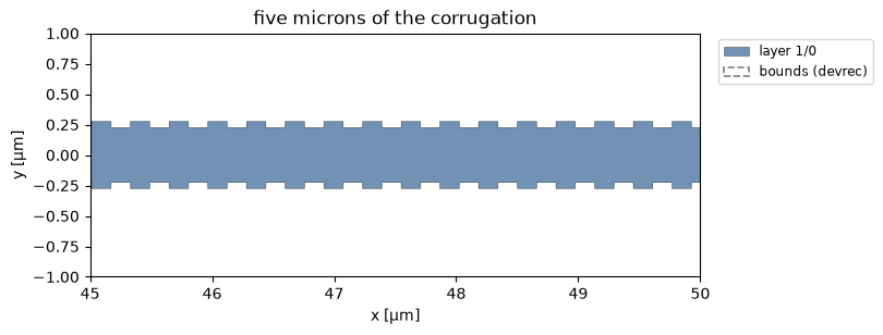
At full scale the grating looks like a plain strip — the corrugation is tens of nanometers on a 95 µm device. Zoom in on a few microns and the periodic teeth appear:

fig, ax = plot_component(comp)
ax.set_xlim(45, 50)
ax.set_ylim(-1.0, 1.0)
ax.set_title("five microns of the corrugation")
plt.show()

1 · One spec: a fine spectrum, a frugal field monitor

Resolving a 3-nm stopband needs a dense wavelength grid — 501 points (0.2 nm spacing) across 1.50–1.60 µm here. Recording the field at all 501 points would multiply the download for nothing, so the monitor keeps seven wavelengths: a tight 0.3-nm comb centered on the Bragg wavelength (1.5430 µm, measured from a first coarse pass on the same mesh) plus two far-out-of-band companions. The z-plane is pinned to the middle of the silicon core:

spec = SimulationSpec(
    wavelength_start=1.5, wavelength_end=1.6, wavelength_points=501,
    mesh=10, z_min=-1.0, z_max=1.0,
    field_monitors=("z",),
    field_monitor_positions={"z": 0.11},
    field_monitor_wavelengths=(1.5424, 1.5427, 1.5430, 1.5433, 1.5436, 1.51, 1.59),
)
solver = get_solver("tidy3d")(comp, technology=tech, spec=spec)
plot_monitor_planes(solver)
plt.show()

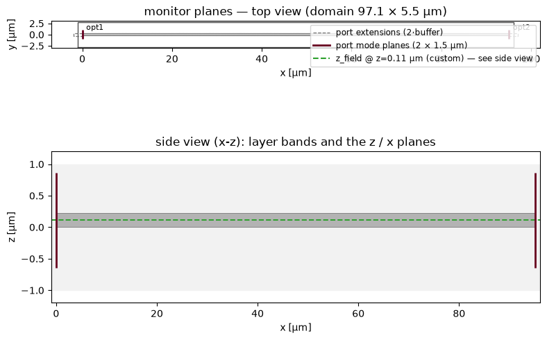
The whole problem in 3D — 95 µm of corrugated silicon in its oxide, the port cones, the pinned monitor plane, and the domain box (orbit / zoom / click):

from gds_fdtd.viewer3d import show_3d  # noqa: E402

show_3d(solver, height=440)

2 · The spectrum

The run executed on tidy3d (2 excitations, ~0.5 FC; artifacts in recorded/, see PROVENANCE.md). Transmission collapses inside the stopband while reflection rises to ~0 dB — a distributed mirror:

sm = SMatrix.from_npz(REC / "bragg_tidy3d.npz")
p_in, p_out = sm.port_names[0], sm.port_names[1]
wl = sm.wavelength_um
s21 = 10 * np.log10(np.abs(sm.sel(p_out, p_in, 1, 1)) ** 2)
s11 = 10 * np.log10(np.abs(sm.sel(p_in, p_in, 1, 1)) ** 2)

order = np.argsort(wl)
wl, s21, s11 = wl[order], s21[order], s11[order]
i_min = int(np.argmin(s21))
lam_bragg = wl[i_min]

fig, ax = plt.subplots(figsize=(8, 4.5))
ax.plot(wl, s21, label=f"S({p_out}←{p_in}) through", color="tab:blue")
ax.plot(wl, s11, label=f"S({p_in}←{p_in}) reflection", color="tab:red")
ax.axvline(lam_bragg, color="0.5", ls=":", lw=1)
ax.annotate(f"λ_B ≈ {lam_bragg:.4f} µm\n(S21 = {s21[i_min]:.1f} dB)",
            xy=(lam_bragg, s21[i_min]), xytext=(lam_bragg + 0.012, s21[i_min] + 8),
            arrowprops={"arrowstyle": "->", "color": "0.4"}, fontsize=9)
ax.set_xlabel("wavelength [µm]")
ax.set_ylabel("|S|² [dB]")
ax.set_title(f"{comp.name}: transmission and reflection")
ax.legend(loc="center right", fontsize="small")
ax.grid(alpha=0.3)
plt.show()

in_band = float(wl[i_min])
below = s21 < -10
if below.any():
    bw_nm = 1000 * (wl[below].max() - wl[below].min())
    print(f"stopband center ≈ {in_band:.4f} um; width (S21 < -10 dB) ≈ {bw_nm:.1f} nm")

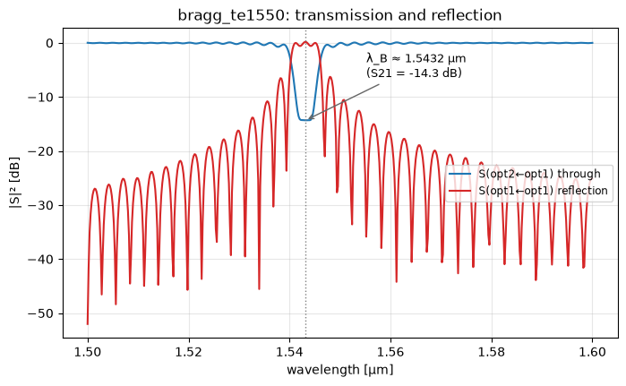
stopband center ≈ 1.5432 um; width (S21 < -10 dB) ≈ 3.6 nm

3 · The same monitor, exactly on the Bragg wavelength

The recorded field file carries the comb; the plot picks the recorded wavelength nearest the spectrum’s own minimum — within the 0.2 nm resolution of the sweep, that is the Bragg wavelength — against the farthest out-of-band companion. In-band, the field decays into the grating — the input side carries a standing-wave ripple where the injected and reflected waves interfere, and almost nothing reaches the output. Out-of-band, the envelope runs flat through all 95 µm:

fz = np.load(REC / "bragg_field_z.npz")
wls = np.asarray(fz["wavelength_um"])
i_in = int(np.argmin(np.abs(wls - in_band)))
i_out = int(np.argmax(np.abs(wls - in_band)))
outlines = component_outlines(comp, axis="z", buffer=2 * spec.buffer) + port_plane_outlines(
    comp, spec, axis="z"
)

fig, axs = plt.subplots(2, 1, figsize=(10, 5.5), sharex=True)
for ax, idx, tag in (
    (axs[0], i_in, "IN the stopband — reflected"),
    (axs[1], i_out, "outside the stopband — transmitted"),
):
    plot_field(
        fz["mag2"][idx], x=fz["h"], y=fz["v"], scale="db",
        ax=ax, outline=outlines, colorbar=False,
        title=f"|E|² dB at {wls[idx]:.3f} µm — {tag}",
    )
fig.tight_layout()
plt.show()

4 · Sanity: energy has to go somewhere

In a lossless reflector, in-band light that does not transmit must reflect. |S11|² + |S21|² stays near one across the band. The dips at the stopband edges are real radiation from the corrugation; the slight overshoot above one at the reflection peak is mesh-10 discretization error (the same few-percent passivity slack the beamz end-to-end test documents) — a finer mesh pulls it in at proportionally higher cost:

balance = 10 ** (s11 / 10) + 10 ** (s21 / 10)
fig, ax = plt.subplots(figsize=(8, 3))
ax.plot(wl, balance, color="tab:green")
ax.axhline(1.0, color="0.6", ls="--", lw=1)
ax.set_xlabel("wavelength [µm]")
ax.set_ylabel("|S11|² + |S21|²")
ax.set_ylim(0, 1.2)
ax.grid(alpha=0.3)
plt.show()
print(f"power balance: min {balance.min():.3f}, max {balance.max():.3f}")

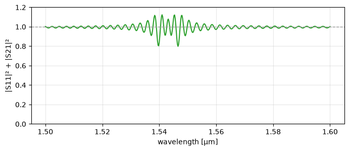
power balance: min 0.799, max 1.123

Recap

• bragg_te1550 from devices.gds, straight from GDS to a tidy3d run with the shared technology file — nothing device-specific in the setup.

• One simulation produced the full 501-point spectrum and the field at seven chosen wavelengths (spec.field_monitor_wavelengths) — a 0.3-nm comb on the Bragg wavelength plus out-of-band companions — pinned to the silicon core (spec.field_monitor_positions).

• The spectrum finds the stopband; the field pictures show why: in-band the grating is a mirror (decay + standing wave), out-of-band it is just a waveguide.