Setting Up Simulations

From a GDS layout to S-parameters in four steps, on any engine.

1. Load the layout

from gds_fdtd.technology import Technology
from gds_fdtd.lyprocessor import load_cell
from gds_fdtd.simprocessor import load_component_from_tech

tech = Technology.from_yaml("examples/tech.yaml")
cell, layout = load_cell("examples/devices.gds", top_cell="crossing_te1550")
component = load_component_from_tech(cell=cell, tech=tech)

Ports are auto-detected from the SiEPIC pin convention (never hand-placed). gdsfactory (>= 9) components convert directly:

import gdsfactory as gf
from gds_fdtd.layout.gdsfactory import from_gdsfactory

gf.gpdk.PDK.activate()
component = from_gdsfactory(gf.components.straight(length=5), tech)

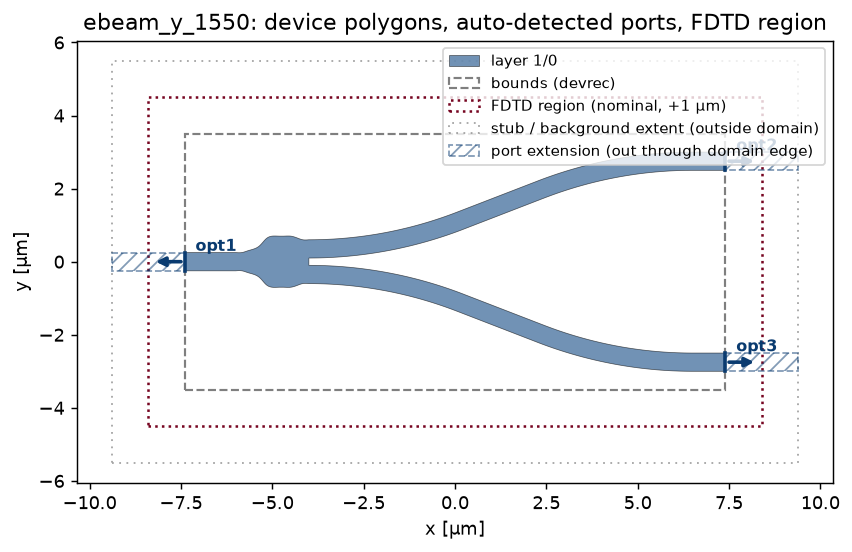
plot_component(component, spec=spec) shows what you loaded, device polygons, the auto-detected ports, the DevRec bounds, and the FDTD region:

2. Configure with SimulationSpec

Every numeric setting lives in one validated model (lengths in µm, angles in degrees, frequencies in Hz, package-wide):

from gds_fdtd.spec import SimulationSpec

spec = SimulationSpec(
    wavelength_start=1.5,
    wavelength_end=1.6,
    wavelength_points=51,
    mesh=10,                      # grid cells per wavelength
    boundary=("PML", "PML", "Metal"),
    symmetry=(0, 0, 0),
    z_min=-1.0,
    z_max=1.11,
    modes=(1, 2),                 # TE + TM
    field_monitors=("z",),
)

Bad values fail loudly at construction with the offending field named.

Field monitors are steerable: one plane per axis in field_monitors ("z" top view, "y"/"x" side views), each sitting at the domain center (x/y) or the device layers’ average mid-plane (z) unless field_monitor_positions pins it to an absolute coordinate. On tidy3d, field_monitor_wavelengths restricts what the monitors record, so a dense S-parameter spectrum does not force an equally dense field download. See where every plane sits before running anything:

spec = SimulationSpec(
    field_monitors=("y", "z"),
    field_monitor_positions={"z": 0.11},      # pin to the Si-core mid-plane
    field_monitor_wavelengths=(1.545, 1.59),  # record just these [um]
)

from gds_fdtd.plotting import plot_monitor_planes
plot_monitor_planes(solver)   # offline: domain, layers, every plane labelled

05b · Field monitors: where they sit, what they record walks through the placement machinery on the Si→SiN escalator, and 11 · A Bragg grating: the stopband, seen in the field uses the wavelength selection to watch one device reflect in-band and transmit out-of-band from a single run.

The whole setup also renders as an interactive 3D scene — the extruded layer stack with per-layer colors, the port cones, each port’s mode plane at its real width_ports × depth_ports (with a dimensions label), the extension stubs, the monitor planes, and the domain box; orbit, zoom, click an object for its material and z-extent, and toggle groups from the legend:

from gds_fdtd.viewer3d import show_3d, save_3d, render_static

show_3d(solver)                     # notebooks AND these docs (three.js)
save_3d(solver, "device_3d.html")   # standalone shareable page
render_static(solver)               # matplotlib, for JS-free contexts

The scene shows true 1:1:1 proportions by default (a 220 nm layer really is hair-thin beside a many-µm device); the legend’s z ×4 checkbox exaggerates the vertical axis when you want to inspect a thin stack. render_static draws the identical scene with matplotlib for the README and other JS-free contexts:

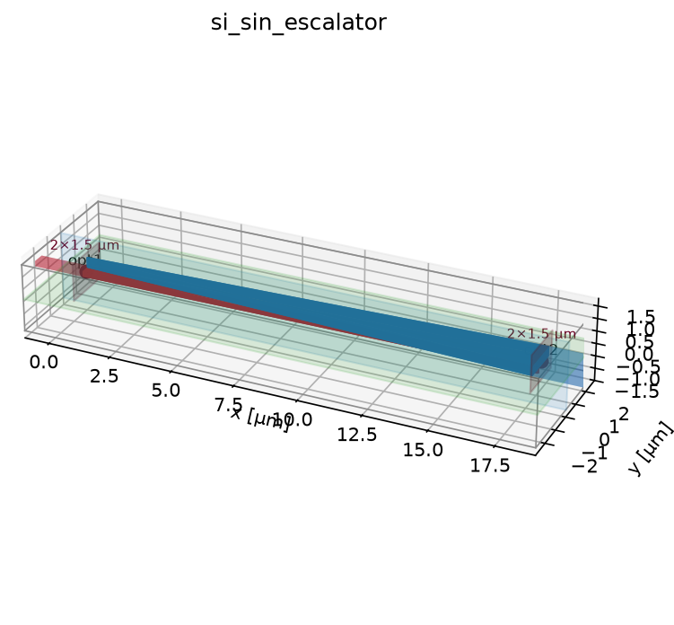
render_static of the Si→SiN escalator solver: the two cores, the translucent cladding, the port mode planes, the monitor planes, and the domain box — the same scene show_3d renders interactively.

The 3D views embedded in 01 · From a GDS layout to a Component, 05b · Field monitors: where they sit, what they record, and 11 · A Bragg grating: the stopband, seen in the field are live — try them.

3. Validate, build, estimate, all free

from gds_fdtd.solvers import get_solver

solver = get_solver("tidy3d")(component, technology=tech, spec=spec)
print(solver.describe())
assert solver.validate() == []
artifacts = solver.build()       # offline: full native scene / setup script
print(solver.estimate())

Nothing so far cost anything: no cloud tasks, no license checkout.

4. Run and analyze

smatrix = solver.run()                        # the only spending step
smatrix.is_reciprocal(), smatrix.is_passive() # physics checks
smatrix.to_dat("device.dat")                  # -> INTERCONNECT
smatrix.to_touchstone("device.s4p")           # -> scikit-rf & friends

from gds_fdtd.plotting import plot_smatrix
plot_smatrix(smatrix, kind="db")
solver.plot_fields(axis="z")

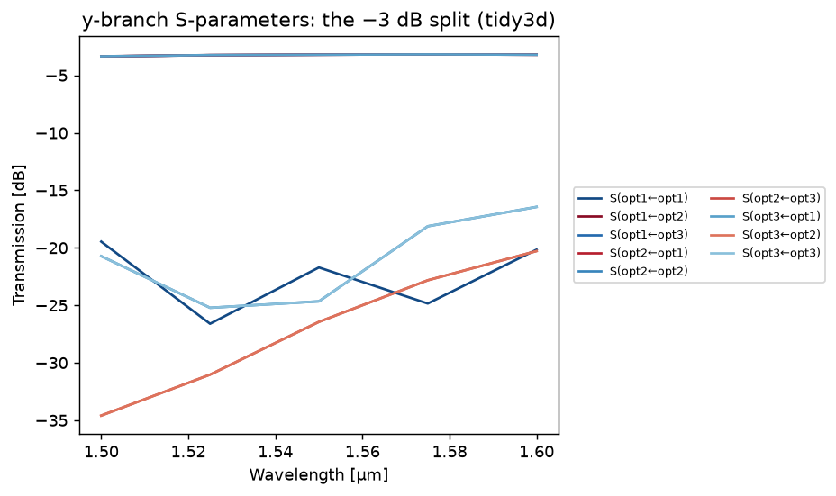
plot_smatrix, every measured path in dB. This y-branch splits its input near −3 dB into each arm.

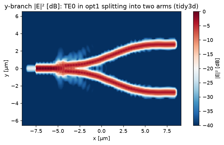
solver.plot_fields(axis="z"), the |E|² field in the device plane, the mode splitting one input into two.

Choosing the mesh

Sweep the mesh and let the S-matrix convergence decide. With a cache directory, repeating a sweep never re-spends:

from gds_fdtd.convergence import sweep

report = sweep(get_solver("tidy3d"), component, tech, spec,
               field="mesh", values=[6, 8, 10], cache_dir=".gds_fdtd_cache")
print(report.summary())
report.recommend(tol_db=0.05)    # first value that moved < 0.05 dB

Ship it anywhere

A simulation is a serializable job; any machine with the package is a worker (see Running gds_fdtd jobs on remote compute):

gds-fdtd validate job.json
gds-fdtd estimate job.json
gds-fdtd run job.json --out results/

Budgets (max_flexcredits / max_wall_seconds) are enforced before and during the run; secrets come from the environment only.